Machine learning/Artificial Intelligence on IBM i

In this article, let’s see a simple machine learning model implemented on IBM i using Python that can predict future values by learning from current data in the system.

As per this article by Gartner, “Data and analytics combined with artificial intelligence (AI) technologies will be paramount in the effort to predict, prepare and respond in a proactive and accelerated manner to a global crisis and its aftermath.” The report goes on to say, “By the end of 2024, 75% of enterprises will shift from piloting to operationalizing AI, driving a 5X increase in streaming data and analytics infrastructures.”

Hence, it is essential to see how we can ready ourselves in the IBM i world to start using these technologies. There are many applications running on the IBM i having a huge amount of data that can be leveraged to get some foresight.

Please note, this article is a demonstration of and not a how-to guide of implementing and running a machine learning algorithm on the IBM i due to the vastness of the subject. For those who are interested to study the subject in detail, I have given links at the end of the article on where and how to start.

I have assumed basic Python programming knowledge. Please refer to my earlier article which demonstrates the use of Python on the IBM i.

Note: The code and data for this article is available to download here.

What is Machine Learning?

As per Google, Machine learning is, “A program or system that builds (trains) a predictive model from input data. The system uses the learned model to make useful predictions from new (never-before-seen) data drawn from the same distribution as the one used to train the model. Machine learning also refers to the field of study concerned with these programs or systems.”

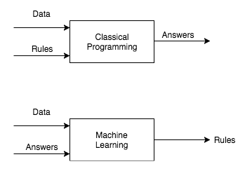
The main difference between traditional programming versus machine learning is as below. We are going to see it in action.

Python libraries we will be using

We will be using the below Python libraries for this task. All the below libraries are already installed on PUB400 globally hence we will not be creating any virtual environment. Please install those if you are trying them on a different server, each library’s documentation provides ways to install those. These are all open-source and free.

1. NumPy

NumPy is a library to handle large, multi-dimensional arrays and matrices. It also supports high-level mathematical functions to operate on these arrays.

2. Pandas

Pandas is a library providing high-performance, easy-to-use data structures and data analysis tools. It offers data structures and operations for manipulating numerical tables and time series.

3. Scikit-learn

Scikit-learn provides a range of supervised and unsupervised machine learning algorithms with a standard interface in Python.

4. Pickle

Pickle is used to save a Python object to a file, for example, a machine learning model which we can load later to make predictions as and when needed.

Some Machine learning terms:

I am giving here a high-level definitions of the terms often used in machine learning so that those will be easy to understand while we build the programs on the system. Please refer to Google’s glossary for more such terms.

1. Features

Features (represented as X) are the parameters using which we will be predicting a value (represented as y). e.g. For predicting the price of a house (y), we will be using parameters such as locality, number of bedrooms, area, etc.

2. Labels

Labels are the values (y) we give to the machine learning model to learn the relation between feature and label (X & y). Labels are the actual price of houses in a dataset.

3. Model

A machine learning model is a trained instance of an algorithm. Training here means the input data (Features & Labels) is used to recognize patterns in it. Using this model we can predict patterns/predictions on a new set of data.

4. Supervised and Unsupervised learning

Supervised learning means when the model is provided with both features and labels (X & y), that is, we provide some pattern of data to the model. In house price prediction example, the number of bedrooms (X) and price of the house(y).

Unsupervised learning means there is no label and the machine learning algorithm has to identify the pattern in it. e.g. grouping of customers based on their spending, earning power, etc.

5. Training

Training is a process by which ideal parameters for a model are determined.

Our machine learning problem

To keep things simple to understand, we will take a simple dataset that contains Years of Experience as X and Salary as y. Using this dataset, we will build the model to predict salary when we input Years of experience into the model.

Similarly, simple to very complex models can be built on IBM i, few examples that come to my mind are:

1. Future raw material requirement.
2. Analyzing quality of material from their images using Convolution Neural Network.
3. Future Revenue prediction based on the past data.

Likewise, the possibilities are endless.

Implementation and testing of the algorithm

Dataset:

We will use a dataset from Kaggle which hosts many data science and machine learning datasets, code, and environments. In a typical environment on IBM i, we will be using data from the system itself, but since this is just a demonstration so any data should give an idea about the concept.

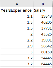
Our data is a file named ‘Salary_Data.csv’ which contains just 31 records including a header row.

Below are just few rows from our dataset.

Linear Regression:

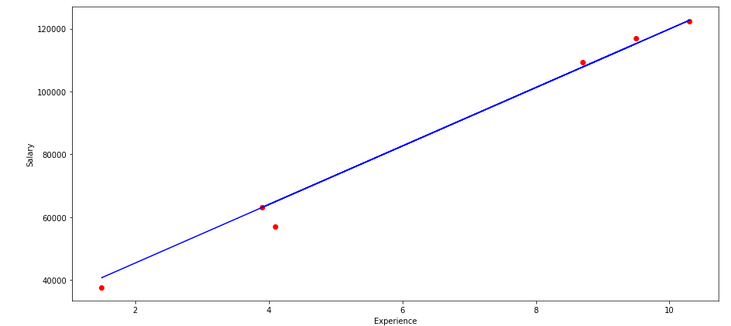
I just want to give a small introduction to the algorithm. When we are working with only one input variable, it is termed Simple Linear Regression. It attempts to find the relationship between two variables using a linear equation.

The linear equation is y=mx + b. Here we are predicting y by fitting the m, which is the slope of the line, and b, which is the y-intercept. Here we have x - years of experience as input.

The graph of which can be plotted as below.

The algorithm tries to find out m and b by minimizing the error when compared to values given in our labels y. An algorithm named Gradient Descent is used to arrive at the values of m and b.

Program:

Let’s see the implementation of the program.

First, we will write a program that will take the data, assign it to X and y variable, split it into the Train and Test set, and then it is used to train the model.

The code for trainmodel.py is as below. Please go through the comments to understand each line.

Change your current directory to ibmi-ml and call the program using the command python3 trainmodel.py.

$ cd ibmi-ml
$ python3 trainmodel.py

You should get the below messages after successful run.

$ python3 trainmodel.py                                       
Linear Regression model built with score: 0.988169515729126 
Model saved in file finalized_model.sav

# NumPy is used to handle the data to put it in a 2-dimensional array.
import numpy as np
import pandas as pd  # Pandas is used to read the data from database or csv.
# Import the LinearRegression class of Sci-kit learn library.
from sklearn.linear_model import LinearRegression
# Import r2_score to measure the performance of our model.
from sklearn.metrics import r2_score
# Split the data as train and test set to test the model.
from sklearn.model_selection import train_test_split
import pickle  # To save the trained model into a file.

# df is a short form of the dataframe, we read the data from the csv and put it in a pandas dataframe object.
df = pd.read_csv('Salary_Data.csv')

# Reshape the data, meaning take one column, the feature, and put it in a 2-D array in a variable named X.
X = df['YearsExperience'].values.reshape(-1, 1)

# Reshape the data,same for the values we are giving to the model based on which it will predict future values in
# variable y.
y = df['Salary'].values.reshape(-1, 1)

# Split the data into the Train and Test sections so that we can measure the performance of the model.
X_train, X_test, y_train, y_test = train_test_split(
    X, y, test_size=0.2, random_state=0)

# Initialize the Scikit learn LinearRegression Class and fit (train the model with training data)
reg = LinearRegression()
reg.fit(X_train, y_train)

# Use Test data to derive the prediction in y_pred array
y_pred = reg.predict(X_test)

# Print the score of the model by comparing it with predicted value and actual test values.
# Score closer to 1 is better performance.
print(f'Linear Regression model built with score: {r2_score(y_test, y_pred)}')

# Save the model to the disk for future use.
filename = 'finalized_model.sav'
pickle.dump(reg, open(filename, 'wb'))

print('Model saved in file', filename)

To demonstrate data handling by NumPy, here is the content of variable X using Python command print(X). Variable X contains “Years of experience”.

[[ 1.1]
 [ 1.3]
 [ 1.5]
 [ 2. ]
 [ 2.2]
 [ 2.9]
 [ 3. ]
 [ 3.2]
 [ 3.2]
 [ 3.7]
 [ 3.9]
 [ 4. ]
 [ 4. ]
 [ 4.1]
 [ 4.5]
 [ 4.9]
 [ 5.1]
 [ 5.3]
 [ 5.9]
 [ 6. ]
 [ 6.8]
 [ 7.1]
 [ 7.9]
 [ 8.2]
 [ 8.7]
 [ 9. ]
 [ 9.5]
 [ 9.6]
 [10.3]
 [10.5]]

Similarly, our corresponding y variable, “Salary” looks like the below when saved in a 2-dimensional array.

[[ 39343.]
 [ 46205.]
 [ 37731.]
 [ 43525.]
 [ 39891.]
 [ 56642.]
 [ 60150.]
 [ 54445.]
 [ 64445.]
 [ 57189.]
 [ 63218.]
 [ 55794.]
 [ 56957.]
 [ 57081.]
 [ 61111.]
 [ 67938.]
 [ 66029.]
 [ 83088.]
 [ 81363.]
 [ 93940.]
 [ 91738.]
 [ 98273.]
 [101302.]
 [113812.]
 [109431.]
 [105582.]
 [116969.]
 [112635.]
 [122391.]
 [121872.]]

These arrays after splitting into Train and Test sets are passed to the LinearRegression class to its fit method. This method takes the data and finds out the co-relation between it, i.e. the values for m and b.

How to re-use the model

We should be able to re-use the model on a new set of data as and when the business needs it. Hence in the above step, we stored the model in a file that can be used often as shown in the program usemodel.py.

import pickle  # Pickle is used to load the stored state of a python object.

# Pass new value to predict from the loaded model.
exp = float(input('Enter years of experience: '))

filename = 'finalized_model.sav'

# Load the model from the disk
loaded_model = pickle.load(open(filename, 'rb'))

result = loaded_model.predict([[exp]])

print('The new predicted salary is', result[0][0])

Our re-usable machine learning model is ready to serve the users. Call the program using the command python3 usemodel.py.

Limitations:

Since this is a very simple model using just one input variable, the predictions will not match reality beyond a certain limit. For example, if we input experience as 40 years, it will predict the salary as 399283.10, which may not be true. A more complex model needs to be configured for accuracy with more features such as education, domain knowledge, etc. Also, the model needs to be tuned with additional parameters such as regularization, which is an advanced topic.

To keep the scope of the article very basic and simple to understand, those additional techniques are omitted from the article.

How to install and run the programs

1. Download the utility folder from here.
2. In the IFS create directory mkdir ibmi-ml.
3. Upload the content of the folder in IFS in directory ibmi-ml.
4. Login to SSH or CALL QP2TERM session.
5. Change the current directory to ibmi-ml using cd ibmi-ml.
6. Create the model using command python3 trainmodel.py. This is a one-time step.
7. Test the model by inputting various experience levels using python3 usemodel.py

Useful links to learn machine learning

These are some of the links I found useful while learning about these topics. This is not an exhaustive list but good enough to start with.

Courses:

1. Machine Learning by Andrew Ng on Coursera
2. Carnegie Mellon University Lectures - Link
3. Machine Learning Crash Course by Google - Link

Books:

1. Hands-On Machine Learning with Scikit-Learn, Keras, and TensorFlow- Link
2. Python for Data Analysis - Link
3. The Hundred-Page Machine Learning Book - Link

Special Thanks

1. PUB400.COM - Such a fantastic server to try out new things on IBM i.
2. Papaya.io - Web-based image editing tool, very easy and fast for image editing.

Conclusion

Machine learning and Artificial Intelligence are becoming a go-to field for data-analytics, robotics, decision-making in every domain. IBM i has a huge amount of data to its advantage as the applications are running for so many years for Banking, Manufacturing, Supply Chain, and numerous other domains. The availability of an environment (PASE for i) which supports open-source on the system and the vast open-source free-to-use machine learning libraries is a win-win situation for any CIO. These can be leveraged for the better good of business and industry.

As always, request you to get in touch with me on LinkedIn/Twitter or email with your valuable feedback. Thanks for reading!